Set Up and Run a Simulation

A good thing when working with the eELib would be the familiarization with the test scenarios of the eELib:

• For a single building to see the operation of devices inside the household.

  • One is with just a few devices and explained setup (“minimum example”),

  • One is for more devices and also using helper functions to create entities, connections etc.

• For a small and simple 8-bus low-voltage grid (2 feeders with six resp. two households) to estimate of the impact of different operating strategies on the local grid.

• For a multi-family household with an energy management orchestrating the coordination between the various households.

With the following explanations of the setup of simulations, try to understand the given examples. Afterwards, you should know what is needed for a simulation and how you could set it up.

What files are needed for a simulation?

To run a simulation, we need just two files: A scenario script and the scenario input data. The input data consists of the model data, the grid information, grid parameters, and the model connections. Additionally, corresponding data such as files for the input of pv generation or a household baseload, must be provided.

Scenario script

Start the simulators, build the models, create the connections and start mosaik. Exemplary scripts for building, grid etc. can be found in the examples folder. The setup of these scripts is explained below in the Scenario Script Configuration section.

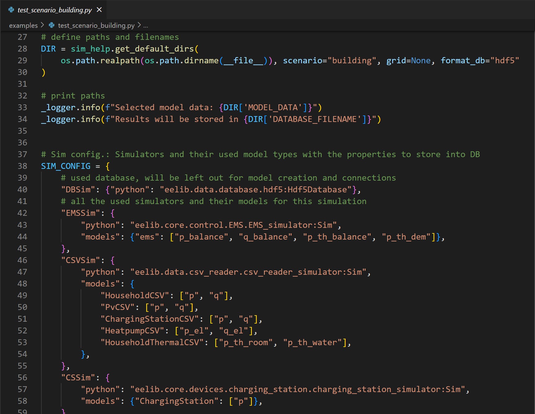
examples/test_scenario_building.py (01/24)

Input data file

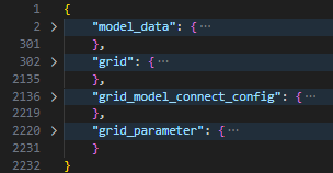
As mentioned before, the input file combines the configuration and parameterization information for the scenario:

• Model data: Information on the number of models and their parameterization.

• Grid: Full details on the given buses and their connections via grid lines and transformer.

• Model connections: Information on linking the model entities in the simulation.

• Grid parameterization: Setup to analyze the grid, limits for buses, lines and transformer.

examples/input/grid.json (02/25)

Model data

Here, the model entites of all model types and their parameterization is stored. E.g. the field “HouseholdCSV” has a dict of all household baseloads (with their naming) that read from a csv file. Have a look at the example below.

examples/input/grid.json (02/25)

{
   "model_data": {
      "PvCSV": {
         "PvCSV_0": {
               "p_rated": 8000,
               "cos_phi": 0.9,
               "datafile": "examples/data_input/pv/pv_10kw_15min.csv",
               "date_format": "YYYY-MM-DD HH:mm:ss",
               "start_time": "2022-01-01 00:00:00",
               "header_rows": 1
         },
         ...
      },
      "HouseholdCSV": {
         "HouseholdCSV_0": {
               "p_rated": 4500,
               "datafile": "examples/data_input/load/baseload_htw_12.csv",
               "date_format": "YYYY-MM-DD HH:mm:ss",
               "header_rows": 1,
               "start_time": "2010-01-01 00:00:00"
         },
         ...
      },
      ...
      "HEMS_default": {
         "HEMS_default_0": {
               "cs_strategy": "max_p",
               "bss_strategy": "surplus"
         },
         ...
      },
      ...
   },
   ...
}

Grid

In .json format (possibly created via pandapower). Provides details on the given buses and their connections via grid lines (plus their parameterization). In case you might be using powerfactory this should be just a path to the grid file that can be used in the powerfactory application (.dz format).

examples/input/grid.json (02/25)

{
   ...
   "grid": {
      "_module": "pandapower.auxiliary",
      "_class": "pandapowerNet",
      "_object": {
         "bus": {
            "_module": "pandas.core.frame",
            "_class": "DataFrame",
            "_object": "{\"columns\":[\"name\",\"vn_kv\",\"type\",\"zone\",\"in_service\"],\"index\":[0,1,2,3,4,5,6,7,8,9,10,11,12,13,14,15,16,17],\"data\":[[\"Trafostation_OS\",10.0,\"b\",null,true],[\"main_busbar\",0.4,\"b\",null,true],[\"MUF_1_1\",0.4,\"n\",null,true],[\"loadbus_1_1\",0.4,\"b\",null,true],[\"KV_1_2\",0.4,\"b\",null,true],[\"loadbus_1_2\",0.4,\"b\",null,true],[\"MUF_1_3\",0.4,\"n\",null,true],[\"loadbus_1_3\",0.4,\"b\",null,true],[\"KV_1_4\",0.4,\"b\",null,true],[\"loadbus_1_4\",0.4,\"b\",null,true],[\"MUF_1_5\",0.4,\"n\",null,true],[\"loadbus_1_5\",0.4,\"b\",null,true],[\"KV_1_6\",0.4,\"b\",null,true],[\"loadbus_1_6\",0.4,\"b\",null,true],[\"MUF_2_1\",0.4,\"n\",null,true],[\"loadbus_2_1\",0.4,\"b\",null,true],[\"KV_2_2\",0.4,\"b\",null,true],[\"loadbus_2_2\",0.4,\"b\",null,true]]}",
            "orient": "split",
            "dtype": {
            "name": "object",
            "vn_kv": "float64",
            "type": "object",
            "zone": "object",
            "in_service": "bool"
            }
         },
         "load": {...},
         ...
      }
   },
   ...
}

Model connections

This includes the connections between grid buses, ems models, and the prosumer devices. It states which devices are located at which grid connection point (by naming the corresponding load bus) and whether an EMS is used. If no EMS is given at a loadbus (see “load_1_3” below), the devices are connected to the grid by a GCP_Aggregator_HEMS that only adds up the power values of listed devices but has no control ability. Hence, this should only be possible for some of the devices, as e.g. a single heat pump with no control makes no sense.

This section also lists the connection from EVs to their charging points, as within one household (especially multi-family houses) there may be more than one CS in a household. If such data is available, this would also allow for public charging points to be included.

examples/input/grid.json (02/25)

{
   ...
   "grid_model_connect_config": {
     "load_1_1": {
         "ems": "HEMS_default_0",
         "entities": [
             "HouseholdCSV_0",
             "ChargingStation_0",
             "EV_0"
         ],
         "cs_ev_connection": {
             "ChargingStation_0": ["EV_0"]
         }
     },
     "load_1_2": {
         "ems": "HEMS_default_1",
         "entities": [
             "HouseholdCSV_1",
             "HouseholdThermalCSV_0",
             "Heatpump_0"
         ],
         "cs_ev_connection": {}
     },
     "load_1_3": {
         "ems": "",
         "entities": ["PVLibExact_0"],
         "cs_ev_connection": {}
     },
     ...
   },
   ...
}

Grid parameters

To set limits for the components in the grid (e.g. buses or lines), you can use this. These values are used to compare the grid results to. Hence, they are net directly set to the grid, as a congestion should be allowed for the power flow to calculate. It should then afterwards be found in the analysis of that results.

examples/input/grid.json (02/25)

{
   ...
   "grid_parameter": {
     "line_loading_max": 100,
     "trafo_loading_max": 100,
     "bus_vm_max_lv": 1.1,
     "bus_vm_min_lv": 0.9,
     "bus_vm_max_mv": 1.1,
     "bus_vm_min_mv": 0.9,
     "bus_vm_max_hv": 1.1,
     "bus_vm_min_hv": 0.95,
     "bus_vm_max_ehv": 1.1,
     "bus_vm_min_ehv": 1.0
 }
}

---

Configuration of a Scenario Script

Tip

The following explanations are just to show and explain what is done to set up a simulation scenario, within the script that you might execute. Although you can configure you scenario script by setting it up with these instructions, it can be a lot easier to use our Scenario Configurator that is introduced in the upcoming sections.

Note

All of these code-blocks derive from examples/test_scenario_building.py as of (02/25) if not stated otherwise.

Setup

import of used packages (examples, like mosaik or logging during the simulation)

import os
import mosaik
import eelib.utils.simulation_helper as sim_help
from eelib.model_connections.connections import get_default_connections
import logging

Setting of paths for simulation data and used model simulators

# define paths and filenames
DIR = sim_help.get_default_dirs(
    os.path.realpath(os.path.dirname(__file__)), scenario="building", format_db="hdf5"
)

Define simulators and models for the simulation

# Sim config.: Simulators and their used model types with the properties to store into DB
SIM_CONFIG = {
   # used database, will be left out for model creation and connections
   "DBSim": {"python": "eelib.data.database.hdf5:Hdf5Database"},
   ...
   # all the used simulators and their models for this simulation
   "HEMSSim": {
      "python": "eelib.core.control.hems.hems_simulator:Sim",
      "models": {
            "HEMS_default": ["p_balance", "p_demand", "p_generation"]
      },
   },
   "CSVSim": {
      "python": "eelib.data.csv_reader.csv_reader_simulator:Sim",
      "models": {
            "HouseholdCSV": ["p", "q"],
            "PvCSV": ["p", "q"],
            ...
      },
   },
   ...

This is done in a format that fits both mosaik for orchestrating the simulation and the handling of data and the simulation setup. So in the “SIM_CONFIG” dict we first need to give all used simulators as the keys (e.g., “CSVSim” for all used csv readers). With the sub-key “python” , we then provide the path to this simulator in our library (e.g., “eelib.data.csv_reader.csv_reader_simulator:Sim”). Under “models” we list all of the used model types within the simulation for this simulator (e.g., “HouseholdCSV”, “PvCSV”) and the attributes of them that should be stored within the database (e.g., [“p”, “q”] for active and reactive power of the PV system).

Configure start and end time of the simulation, step length, and whether to use forecasts. Model data and connections are read and SIM_CONFIG is handed to mosaik.

# Configuration of scenario: time and granularity
START = "2020-01-01 00:00:00"
END = "2020-01-04 00:00:00"
USE_FORECAST = False
STEP_SIZE_IN_SECONDS = 900  # 1=sec-steps, 3600=hour-steps, 900=15min-steps, 600=10min-steps
N_SECONDS = int(
    (
        arrow.get(END, "YYYY-MM-DD HH:mm:ss") - arrow.get(START, "YYYY-MM-DD HH:mm:ss")
    ).total_seconds()
)
N_STEPS = int(N_SECONDS / STEP_SIZE_IN_SECONDS)
scenario_config = {
    "start": START,  # time of beginning for simulation
    "end": END,  # time of ending
    "step_size": STEP_SIZE_IN_SECONDS,
    "n_steps": N_STEPS,
    "use_forcast": USE_FORECAST,
    "bool_plot": False,
}

# Read Scenario file with data for model entities
with open(DIR["INPUT_DATA"]) as f:
    scenario_data = json.load(f)

# Read configuration file with data for connections between prosumer devices
model_connect_config = get_default_connections()

# Create world
world = mosaik.World(SIM_CONFIG, debug=True)

With mosaik.World, we start the orchestrator mosaik and afterward set up the simulation using mosaik. For this, we mostly use mosaik functionalities within the helper functions of the eelib.utils.simulation_helper folder. Regarding the order, we mostly first handle the exceptions of the models, like the output database, and afterward use the helper functions for all other models. Fore a deeper understanding of what is done with these steps, you should look at the implementation of these helper functions and possibly even the setup of mosaik for creating the simulation.

---

Start Simulators for all used Models

# start all simulators/model factories with mosaik for data given in SIM_CONFIG
dict_simulators = sim_help.start_simulators(
    sim_config=SIM_CONFIG, world=world, scenario_config=scenario_config
)

---

Initiate Model Entities using the created Simulators for each Device Type

# create all models based on given SIM_CONFIG
dict_entities = sim_help.create_entities(
    sim_config=SIM_CONFIG, model_data=scenario_data["model_data"], dict_simulators=dict_simulators
)

---

Connect Entities

The connections for each entity are listed in the model_connect_config data. Now tell mosaik about them and let mosaik create graphs for how the calculation procedure of the simulation is to be executed. Additionally, the entities are connected to the database to store the desired resulting property values.

# connect all models to each other
sim_help.connect_entities(
    world=world,
    dict_entities=dict_entities,
    model_connect_config=model_connect_config,
    dict_simulators=dict_simulators,
)

---

Run Simulation

world.run(until=scenario_config["n_steps"], print_progress=True)

Just go Ahead and Run a Simulation

• You can run one of the test_scenarios in the examples folder

• While running the simulation, some stuff is logged like creation of simulators, entities, and connections. Additionally, mosaik plots the progress of the whole simulation (like how many time steps are finished calculating).

• Adapting the parameterization in the simulation files can yield quite different results.

• Running one of the simulations will create a .hdf5 results data file in the folder /examples/results.

• You can view the information of this file via the H5Web Extension in Microsoft VSC and plot the profiles (stored under Series) of the used devices.

• If you want, you can set the parameter bool_plot in the scenario_config dict to true (only do this for small simulations!). mosaik will then present four plots for the connections, the simulation process and the timely duration during the simulation.

Configure a Simulation Scenario

For sure, you may create your own simulation by simply

• Copying one of the scenario scripts,

• Deleting all of the redundant stuff (simulators/devices/connections), and

• Copying and setting up the corresponding input file.

ALTERNATIVELY, you can (or should!) use our easy …

Step-by-Step Scenario Configurator

To create all the needed files for your own scenario, you can use the jupyter notebook script_sim_setup.ipynb in the subfolder eelib\\utils\\simulation_setup. In this notebook you will be guided through all the steps of setting up your simulation scenario. Those steps will be shortly explained here, for more information just have a look at the notebook, which aims to be self-explanatory.

1. Generate model overview: You can create an .rst file that displays all the models of the eELib and their parameters.

2. You can create your local power grid with different options:

   • Use a pre-defined Pandapower or SimBench grid.

   • Create an easy radial LV grid.

   • For using PowerFactory, you should just provide the path to your grid file.

3. Set parameters for the grid including limits for buses, lines and transformer.

4. Generate the model data: You can create and set all your model entities including their parameterization within excel files, again using different options:

   1. All models should have the same parameterization, then you have to give that configuration once and afterwards list, at which grid loads these models should be connected.

   2. The models can have different parameterization, then you have to list them specifically.

5. Create the full input file for your scenario.

6. Finally, if you set the last configuration parameters, you can also create the script to execute your scenario. Optionally, you can shift the scenario files to the examples folder so you just have to press play to execute your own scenario.